3 Spatial exante profitability and risk toolkit
3.1 Spatial parametric production function approach with risk
Purpose: The conventional approach is to estimate a parametric production function (also called crop response function), then use profit maximization or it’s dual cost minimization to identify optimal demand for the associated technology. If risk is considered important, the traditional approach is to assume a quadratic utility function and use mean-variance approaches to assess optimal choices under risk aversion preferences (e.g., Just-Pope production function or moments productions). To use this approach for spatial exante, we use spatial Bayesian models for point-referenced data (Note: spatial econometric approaches can also be used for this extension to the traditional model).
Advantages
- Simple to use with standard econometric approaches (e.g., OLS).
Disadvantages
- Difficult to identify the appropriate functional form and the results are largely dependent on this choice.
Stylized use case: Are sowing date advisories risk proof?
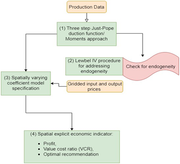
We use CSISA-KVK trial data to understand whether early sowing of wheat and planting of long duration wheat varieties increase mean yield and reduce risk. Workflow Figure 4 shows a workflow for the spatial parametric production function approach. This is categorized into four steps. First, one estimates a production risk function model using either the residual based (e.g., Just-Pope production function) or the moments-based approach using ordinary least squares approach. If there are concerns with endogeneity, then one can correct for these using the instrumental variables approach or other quasi-experimental methods. The simple approach we recommend is using Lewbel (2012) approach. Third, to make the estimate spatially explicit, we recommend using a spatially varying coefficient model to get estimates for each pixel in area of interest. Finally, one can use input and output prices to create economic indicators of interest.
Replication materials: https://eia2030-ex-ante.github.io/SpatialParametricProduction_Risk_Model/
Key references:
Antle, J.M. 1983. “Testing the stochastic structure of production: A flexible moment-based approach”. Journal of Business and Economic Statistics 1(3): 192-201. Doi: 10.1080/07350015.1983.10509339.
Antle, J.M. 2010. “Asymmetry, partial moments and production risk.” American Journal of Agricultural Economics 92(5): . Doi: https://doi.org/10.1093/ajae/aaq077.
Di Falco, S., Chavas, J., and Smale, M. 2007. “Farmer management of production risk on degraded lands: the role of wheat variety diversity in the Tigray region, Ethiopia.” Agricultural Economics 36: 147-156. Doi: https://doi.org/10.1111/j.1574-0862.2007.00194.x.
Di Falco, S., and Chavas, J. 2009. “On crop biodiversity, risk exposure, and food security in the highlands of Ethiopia”. American Journal of Agricultural Economics 91(3): 599-611. Doi: https://doi.org/10.1111/j.1467-8276.2009.01265.x.
3.2 Causal ML and spatial probabilistic assessment model
Purpose: In some cases, the farmer is not only interested in shifting to a technology that gives the highest yield gains, but also the one that has the highest chance of giving him/her yields beyond a particular threshold.
Advantages
The spatial probabilistic approach adds value under the following circumstances:
One is interested in segmentation of zones of opportunities.
One is interested in threshold probabilities as measures of uncertainty.
Disadvantages
- The spatial Bayesian models are computationally expensive especially for large N data and can take many weeks to produce results. This can be resolved by using High Performance Computers.
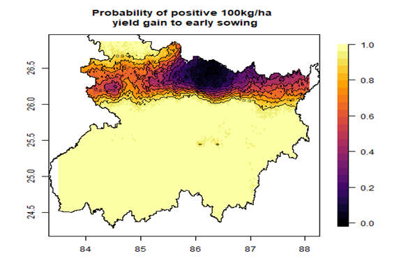
Stylized use case: Where to target sowing date advisories that achieve yield gains beyond a particular threshold?
A farmer requires a substantial yield gain to change from the conventional behaviour. In recommending planting date changes, it is therefore important to provide the confidence we have that the farmer will likely attain yields higher than that threshold. A probabilistic assessment approach allows this through a threshold probability—the probability that a farmer in that location will achieve yield gains above the threshold.
Input data requirements: The approach requires geo-referenced farm plots with attendant yield and traditional production variables (e.g., fertilizer, weed management, e.t.c).
Toolkit workflow
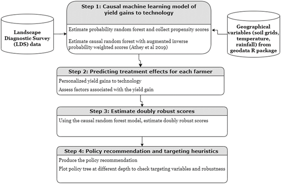
This toolkit is implemented by following the steps shown in the figure 7.
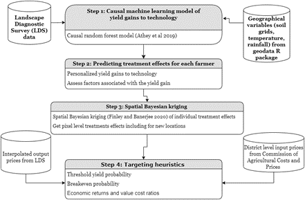
Stylized outputs
Using this toolkit, we see in Figure 8 that farmers in much of the area of interest (Bihar) would find early planting of wheat most beneficial and have a probability of getting an additional 100kg/ha due to early sowing alone.
Replication materials: .https://github.com/EiA2030-ex-ante/CausalML_SpatialBayes_Model. Other interpolations methods can be found here:https://github.com/EiA2030-ex-ante/Interpolation_Kriging_Methods_for_Exante
Key references:
Athey, S., Tibshirani, J., and Wager, S. 2019. “Generalized Random Forests.” The Annals of Statistics 47(2): 1148-1178. Doi: 10.1214/18-AOS1709.
McCullough, E.B., Quinn, J.D., Simons, A.M. 2020. “Profitability of climate-smart soil fertility investment varies widely across sub-Saharan Africa.” Nature Food 3:275-285. Doi: https://doi.org/10.1038/s43016-022-00493-z.
Mkondiwa, M., Hurley, T.M., and Pardey, P.G. 2024. “Closing the gaps in experimental and observational crop response estimates: a bayesian approach”. Q Open 4. Doi: https://doi.org/10.1093/qopen/qoae017.
3.3 Causal ML and policy learning optimization model
Purpose: To make individualized or personalized recommendations from observational data in a data-driven manner using causal machine learning frameworks.
Advantages
- Data-driven approach of recommending alternatives without making functional form assumptions. This is especially useful for agricultural inputs for which we do not have a clear functional form e.g., irrigation, sowing dates.
Disadvantages
- It requires enough sample sizes for each of the options being compared. This mean that for new innovations which have not been extensively adopted, this approach would not be beneficial.
Stylized use case: Targeting sowing date advisories to individual farmers
While sowing date and many other recommendations are made on the basis of climatic, biophysical and economic aspects, there may be several individual level reasons for not following with the recommendation, e.g., family members are busy with other duties during those weeks. We propose a robust methodology that rests on causal machine learning and policy learning to make recommendations that are the most beneficial for each individual farmer.
Input data requirements: The data required is the same as for any conventional production function or impact assessment. These include yield, agronomic management variables (e.g., fertilizer applied), socio-economic variables, and input and output prices. One however, needs enough sample sizes for the treatment and control groups therefore the method works only for a technology which has been widely adopted.
Toolkit workflow
Figure 9 shows a step-by-step workflow for implementing the policy learning optimization model.
Stylized outputs
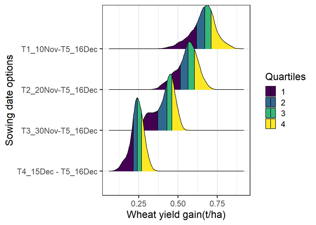
The output of steps 1 to 3 in the workflow are the individual level estimates of the yield gains from the proposed agronomic innovation. Figure 10 shows the distribution of yield gains to early sowing. Everyone in the sample would get a positive yield gain if they advance their planting strategy as compared to sowing after 16 December. The highest yield gains are with planting before 10th November. However, the results in this figure do not prescribe a recommendation for that farmer. To prescribe a recommendation, we need to assume some objective function of the farmer. Policy learning uses minimum regret as an objective function to prescribe best practice for each farmer. Figure 11 then shows the transition matrix from status quo to proposed agronomic practice for each individual farmer.
![]()
Replication materials: https://eia2030-ex-ante.github.io/causal_RF_targeting/ for an application in India and https://github.com/MaxwellMkondiwa/TZ_Spatial_NUE_Trends_Causal_AI for an application in Tanzania.
Key references
Athey, S., and Wager, S. 2021. “Policy learning with observational data”. Econometrica. Url: https://onlinelibrary.wiley.com/doi/abs/10.3982/ECTA15732.